![]()
![]()
![]()
![]()
![]()
![]()
![]()
![]()
![]()
![]()
![]()
![]()
![]()
![]()
Tutorial Page 1
![]()
We will begin by running the simplest experiment, a time series where the changing level of two proteins is plotted against time.
Look at the main program window and it should look something like this.
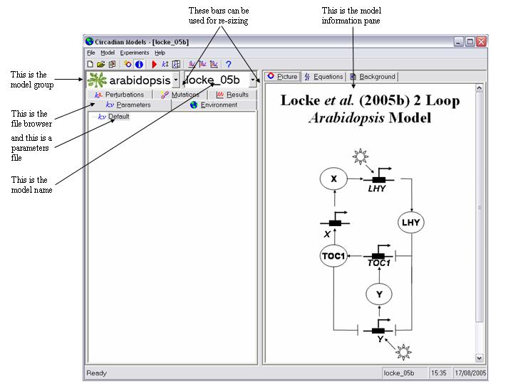
You will see it is divided vertically into two panes. In particular note the two drop down list boxes in the top of the left hand pane. The user interface and the models it contains are separate entities. Before you can use a model it must be installed into the interface. When you installed the program one model will have been installed by default. This is called "locke_05b" and is a model of the Arabidopsis clock developed by our lab and published in Molecular Systems Biology doi: 10.1038/msb4100018. This model has been placed in a model group called "arabidopsis". The purpose of grouping the models is to make them easier to manage and to locate the desired one. This will be especially important when a large number are installed. There is no other significance to this.
- Lets use this model, as at this stage it may be the only one installed. The right pane shows a graphical representation of the model equations. Click on the "Equations" tab to see the actual equations, or the "Background" tab to learn more about the model.
- Every simulation needs a parameters file to run. This contains values for all the constants which appear in the model equations, representing things such as reaction rate constants, together with initial values for all the model states, which are proteins, RNAs etc. Click on the "Parameters" tab of the file browser and you will see the name of the only parameters file present at this stage appear in the browser window. This is called "Default". Double click on its name to open it.