![]()
![]()
Tutorial Page 10
![]()
In this experiment we will look at simulating mutations by manipulating model parameters. We will run the mutation alongside the wild type and compare the results.
The first thing we need to do is to create the mutation. We could simply edit a parameters file directly, but there is a convenient shortcut. Click the "Mutations" tab of the file browser. Right click the file view area and select
Newfrom the popup menu. This will launch the mutations dialogue box.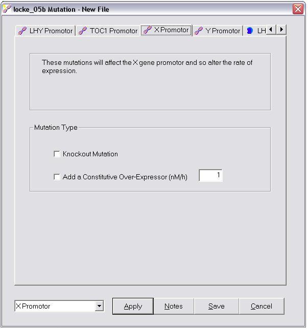
The tabs represent possible targets for mutation, and consist of gene promoters and proteins. On each tab is a list of possible ways to mutate that target. These lists are not exhaustive, but are just the ones I managed to think up when writing the software. Any other mutation can be created by simply editing the parameters file directly.
We are going to add an constitutive copy of the X gene, so click the "X promotor" tab.
Check the "Add a Constitutive Over-Expressor" box to activate this mutation. The value in the box is the rate of expression that this gene will have. Lets leave it at "1".
When adding an over-expressor gene, you may if you wish, knock out the native regulated copy of the gene. This not necessary but we will do it here as an example. Check the "Knockout Mutation" box.
Now click "Save" and save the mutations file under the name "X ox", and click "Close".
So far we have just defined a combination of two mutations. We haven't actually applied them yet. We must do this now by applying the mutations file to a parameters set. Click the "Parameters" tab and open the parameters file "Default". Click "Mutate" and choose the file "X ox" we just created from the list that appears and click "OK".
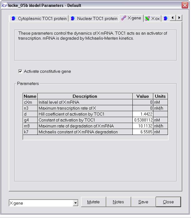
The parameters form will now look like this. The parameters cXm and n3 will be changed to zero and coloured grey. This is the result of the knockout mutation. The colour is just to indicate that they have been affected by the mutation. You can still edit them further if you wish.
Notice also that the "Activate constitutive gene" box is checked and this has resulted in the appearance of a new tab called "X ox".
Click on this tab and you will see the parameters relating to the over-expresser gene that control its transcription and translation.
Now save the file under the name "X ox" and close the form.
We could now run the mutation as it is, but it might be more interesting to cause the over-expresser to be switched on part way through a simulation. This also introduces us to the concept of parameter perturbations. The parameters are not after all constants. They can have their values altered at defined time during a simulation, giving enormous flexibility. To see how this works click on the "Perturbations" tab. Right click on the file view area and select
Newfrom the popup menu. This launches the perturbations dialogue box.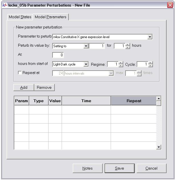
We want to perturb the rate of expression of the constitutive X gene we have added by setting its rate to zero for an initial period.
This is a parameter not a state, so click on the "Parameters" tab. Select "n4ox Constitutive X gene expression level" from the drop down list at the top (it will be somewhere near the bottom of the list).
Set the "Perturb its value by" list to "Setting to", and the values next to it to "0" for "120" hours. The other values you can see determine when the perturbation will begin. Leave them as they are and it will begin at the start of the simulation. Click the "Add" button and the details just entered will appear in the grid below.
Click "Save" and save the file as "X ox off" and click "Close".
The final thing we need to do is create an environment file long enough to apply this mutation. Click the "Environment" tab, open the file "Default" and change the number of cycles to 10. The cycle itself should still be LD 12:12. Save the file.
We are now ready to run the mutation. It could be run as a simple time series experiment, but it might be more interesting to run it alongside the wild type and compare the results. Click the
Experiments->Time
  Series->Compare Simulations->Vary Input File
menu item. This will produce the dialogue box below.
In this module we are saying that we want to run a number of simulations with different input files and compare the results. We choose the files for each run with this form.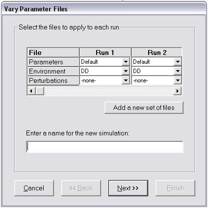
In the "Run 1" column change the environment file to "Default". In the "Run 2" column change the parameters file to "X ox" to use our mutation, change the environment file to "Default", and apply our perturbation by setting the perturbations file to "X ox off".
You can see from this form that unlike parameters and environment files, perturbations files are optional. The default is always "-none-".
Enter a name for the workbook and click "Next".
This form will appear. This is the form we have been ignoring up until now.
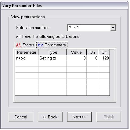
Perturbations files define perturbation times in terms of the environment cycle, not as absolute times. For this reason, perturbation times are not generated until a perturbations file is combined with an environment file. This has now been done and the results are displayed on this form.
Change the "Select run number" box to "Run 2" (Run 1 has no perturbations to see). The grids now show the perturbations that will be applied during this run. There are no state perturbations, so this grid is empty, but as you can see, the parameters perturbation will be applied from zero to 120 hours to parameter n4ox.
Of course in this example as the perturbation was applied at the very start then it makes no difference to the time which environment file is selected.
Click Next to bring up this form.
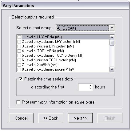
Here we are asked to select the model outputs we are interested in analysing. Check "4 Level of TOC1 mRNA", "7 Level of X mRNA", and "48 Level of X mRNA from constitutive gene".
Ensure the "Retain the time series data" box is checked and click Next.
- You will now see the integration dialogue box again. We won't bother integrating this time. Just click "Finish" to launch the simulation and wait for it to complete.