![]()
![]()
Tutorial Page 9
![]()
A progress bar will now appear. The simulation will probably take a minute or so, depending on the speed of your computer. When this is complete, launch the results workbook.
The first worksheet in the book is again called "Title". This will be the same as before, except that information on the parameter variations between runs is appended at the bottom.
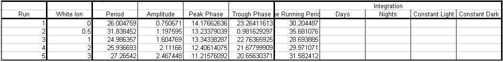
The next worksheet is called "Summary Data". This contains a table comparing how various aspects the output vary between runs. It will look like this.
As you can see, the effect of varying the light intensity on period, amplitude, peak and trough phase and area under the curve for each period is shown. These values represent the values for the final cycle period for each run, except integration which is the next to last. This is because the final integration block is not always the same length as earlier ones, depending on the precise length of the simulation. Integration values appear in the column "Free Running Period" because we elected not to integrate against the light cycle. If we had done so then the same values would appear in the "Constant Light" column. Again these values are all Excel formulae.
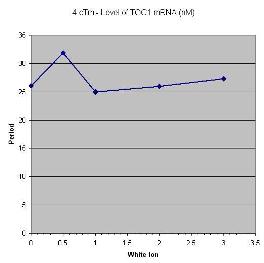
Next is a sheet called "Summary Charts" which contains plots of this data. For example, the effect on light intensity on free running period should look something like this
The next worksheet is called "Environment 1". This contains all the light values for the first run of the simluation. These will be all zeros.
The next worksheet is called "cTm, Run 1". This contains the time series values for the selected output. As before for the simple time series experiment there is a table of peak and trough time values and analysis, a table of integration values, and an embedded plot of the integrated data.
There will be a corresponding pair of these last two sheets for all five runs.
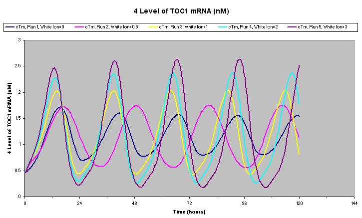
At the end of the book there are two charts. The first "Chart - cTm" is a plot of the five sets of time series values all on the same axes. It should look something like this.
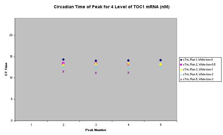
The second chart "Chart - cTM Peaks" is a plot of CT time of each peak time, with a separate series for each run. This is produced because it was possible to calculate CT times in this experiment due to the environment being constant conditions. It should look like this.
Measuring circadian time of the peak is useful because any change of peak time relative to the cycle period may indicate a change in shape of the waveform.
That concludes this experiment. Next we'll take a look at mutations.